Tuning
Speaking of bandwidth, and the second part of your question: how do we chose these gains? As with any filter, the trade-off is lag vs smoothness. The appropriate value depends on the resolution of your encoder and your application. High bandwidth (i.e. aggressive) control requires a high bandwidth state estimate, but the cost is more sharp reactions to encoder pulses.
Higher resolution encoder means each pulse has a smaller magnitude in the “staircase”, so you get less sharp reactions, and hence you can turn up the bandwidth for the same magnitude noise/ringing in the system.
Theory
Okay so do we derive the gains? First of all, we look at the structure of the way the PLL is set up: it’s like a PI loop, which is a 2nd order system. So two important characteristics of a 2nd order system is it’s Bandwidth and Dampening (and frequency, but we won’t need that, as we’ll see later). We will discuss the system response in terms of it’s poles.
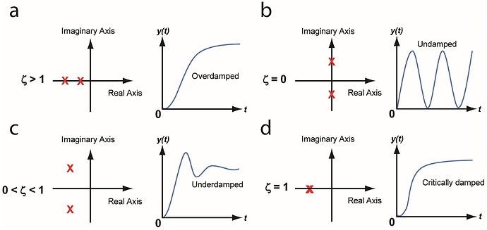
So what exactly are poles? This gets quite involved and there are entire lecture courses about this, but here is some quick intuition: Poles are complex numbers that describe a system behaviour. They either sit on the real axis, or they are in complex conjugate pairs. With real poles, there is no oscillation, no overshoot. With complex conjugate pairs, there can be some ringing, overshooting, or even oscillation. This is summarised nicely here (source):
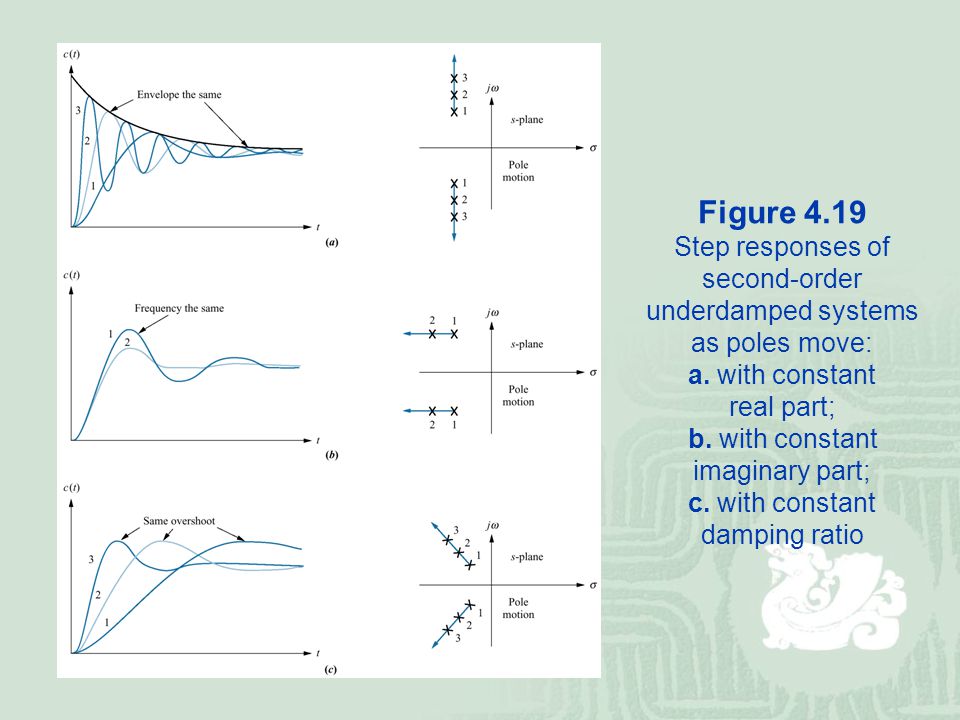
More quantitatively, a pole further to the left is “faster” (higher bandwith), and poles with larger imaginary parts oscillate at a higher frequency. What’s the difference? Again this is best shown with a picture:
Note that in all of this, the units for the location of the poles can be taken as radians/s. So if the pole pair is at -2 ± 5i, then we have a sinusoidal response with a frequency of 5 radians/s, that decays with an envelope of speed 2 rad/s.
So let’s say the blue trace is position in response to a sudden increase in input position, i.e. an encoder input change. Suppose we want the filtered output to track this as fast as possible, without ever overshooting. This happens when the two poles (the red X’s) are exactly on top of each other: this is called critically damped (see bottom right example in 1st picture).
Derivation
I derived it by going backwards: suppose we have some P and I gains (Kp and Ki), what are the poles, and hence what is the bandwidth and how is the damping? I chose to derive it as a continous time system (to be approximated in discrete time) because I was more familiar with that; if someone has the direct discrete-time derivation please do chime in  .
.
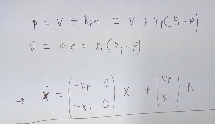
So the equations below we have two states p for position and v for velocity. For clairity I used a variable to e to mean the error between the position state and the encoder reading, the latter designated as p_i for “input position”. We can let a vector x be equal to [p, v], and hence write the two equations in matrix format.
Now you will have to trust me on this: the poles of this system is equal to the eigenvalues of the matrix on the left, the system matrix, commonly called A. (If you don’t trust me, check this).
Okay so what are the eigenvalues of the matrix? Back in the day you would have to go do some algebra, but with modern technology we can have computers do that for us: we use SymPy. Try it yourself at SymPy live. Enter this command: Matrix([[-x, 1], [-y, 0]]).eigenvals(). Pretend that x means Kp and that y means Ki. Voila, the solution is:
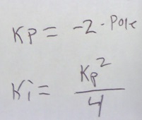
Going back to our specification: we want the real part of the pole to be some specific number, which is our bandwith (in radians/s) and we want the imaginary part to be zero on both poles. Solving for that yields:

Which is exactly what is in the code:
motor->rotor.pll_kp = 2.0f * rotor_pll_bandwidth;
// Critically damped
motor->rotor.pll_ki = 0.25f * (motor->rotor.pll_kp * motor->rotor.pll_kp);
 .
.