Rotor Encoder PLL and Velocity

I am curious if you could explain a bit more about how the PLLs on the encoders work in theory and your implementation. Filtering in controls classes was probably my weaker area for sure and this may be hurting my understanding.
I have been working on a BLDC driver a bit on my own just for fun. (Smaller single axis board one per joint for hopefully what will soon be a nice walking quadruped robot). For my impedance control algorithms I am having a tough time getting good quality velocity estimates especially at low speed. You seem to not have this problem judging by watching the smoothness in the demo videos.

I have been looking at your PLL code and of course like all good implementations it seems really simple in the end. If you could shed some light on how you get to these formulas and how the gains are tuned for different velocity profile needs that would be a huge help! Looking forward to seeing the continued development of this project and hoping this community continues to grow. Bringing this level of capability down to use hobbyist is huge.

Thanks,

So the PLL is basically a state estimator for the rotor angle and rotor speed, using the encoder as measurement. If you want to dig into the theory of this kind of stuff, you should look at the concept of a state observer.

But let’s dig into what’s going on in the code I wrote, and maybe I can indeed shine some light.
The estimator has two states: position and velocity. The position is in encoder counts, and the velocity is in counts/s. Since the encoder keeps counting up as we turn past one full turn, we can imagine the state to be along an unrolled line rather than an angle, and hence we can talk about position (in counts) rather than angle.

So given these two states of position and velocity, the simplest thing we can do is use the velocity to predict the position over time. This is important for interpolating the encoder position between discrete counts. That is, we track with a 1st order (straight line) the expected position at all times, even when we are between encoder pulses. This gives a smoother control, and higher effective precision.
It is also important to predict where the expected angle is so we can predict when we expect the next encoder pulse to come. If it’s late or early, that gives us information about the fact that we over or under estimated the velocity. So: here’s the code for that prediction, super simple 1st order integration of velocity:

// Predict current pos
rotor->pll_pos += CURRENT_MEAS_PERIOD * rotor->pll_vel;

Okay, now we do the part where we check if the encoder edge is early or late. This revolves around a function that takes the predicted angle in full float precision (so like encoder counts with many decimal places), and tells us what encoder count that should correspond to. So like, if the underlying angle is a ramp, the encoder counts will be a staircase. We use the floor function to do this ramp-to-staircase mapping.
So if our predicted angle is a bit behind, and hence our staircase hasn’t stepped to the new step yet, but the encoder has, we are early, and also delta_pos will be 1.0f for as many cycles we are late for, until our prediction has also switched to the next state.

// discrete phase detector
float delta_pos = (float)(rotor->encoder_state - (int32_t)floorf(rotor->pll_pos));

So, we know we are early or late, great, so now we act on that. Suppose we are late, we need to speed up the velocity estimate, which is the second line below. In that second line, we accelerate (increase velocity with a rate) proportional to our position error: just like a mass-spring system. Likewise, without damping, it would form a harmonic oscillator and oscillate around the correct value. So we need to add damping. This is done by stepping the position estimate closer to the measurement by some amount too, hence the 1st line below.
Another way to interpret it is that we have a PI loop that, where the encoder is the input signal that we try to track with some finite bandwidth.

// pll feedback
rotor->pll_pos += CURRENT_MEAS_PERIOD * rotor->pll_kp * delta_pos;
rotor->pll_vel += CURRENT_MEAS_PERIOD * rotor->pll_ki * delta_pos;
5 Likes

Thanks for responding with such a well written post. I had never quite thought about this a ramp function and then like you desribed back to the more discrete stair stepping of the integer world of the true encoder state.
That makes it way more clear how the underlying estimations are done. Thank you!. Look forward to the rest on the gains!

1 Like

Tuning

Speaking of bandwidth, and the second part of your question: how do we chose these gains? As with any filter, the trade-off is lag vs smoothness. The appropriate value depends on the resolution of your encoder and your application. High bandwidth (i.e. aggressive) control requires a high bandwidth state estimate, but the cost is more sharp reactions to encoder pulses.
Higher resolution encoder means each pulse has a smaller magnitude in the “staircase”, so you get less sharp reactions, and hence you can turn up the bandwidth for the same magnitude noise/ringing in the system.

Theory

Okay so do we derive the gains? First of all, we look at the structure of the way the PLL is set up: it’s like a PI loop, which is a 2nd order system. So two important characteristics of a 2nd order system is it’s Bandwidth and Dampening (and frequency, but we won’t need that, as we’ll see later). We will discuss the system response in terms of it’s poles.

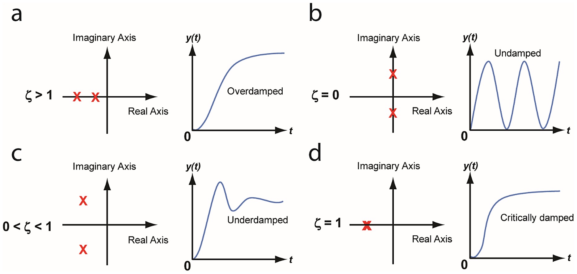
So what exactly are poles? This gets quite involved and there are entire lecture courses about this, but here is some quick intuition: Poles are complex numbers that describe a system behaviour. They either sit on the real axis, or they are in complex conjugate pairs. With real poles, there is no oscillation, no overshoot. With complex conjugate pairs, there can be some ringing, overshooting, or even oscillation. This is summarised nicely here (source):

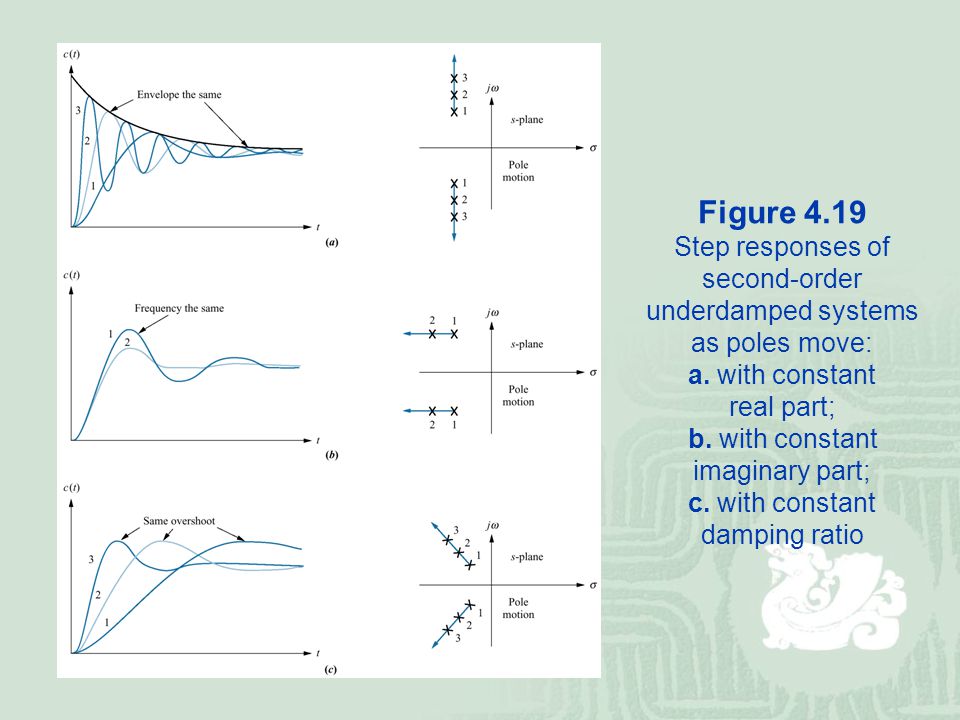
More quantitatively, a pole further to the left is “faster” (higher bandwith), and poles with larger imaginary parts oscillate at a higher frequency. What’s the difference? Again this is best shown with a picture:

Note that in all of this, the units for the location of the poles can be taken as radians/s. So if the pole pair is at -2 ± 5i, then we have a sinusoidal response with a frequency of 5 radians/s, that decays with an envelope of speed 2 rad/s.

So let’s say the blue trace is position in response to a sudden increase in input position, i.e. an encoder input change. Suppose we want the filtered output to track this as fast as possible, without ever overshooting. This happens when the two poles (the red X’s) are exactly on top of each other: this is called critically damped (see bottom right example in 1st picture).

Derivation

I derived it by going backwards: suppose we have some P and I gains (Kp and Ki), what are the poles, and hence what is the bandwidth and how is the damping? I chose to derive it as a continous time system (to be approximated in discrete time) because I was more familiar with that; if someone has the direct discrete-time derivation please do chime in :smiley:.

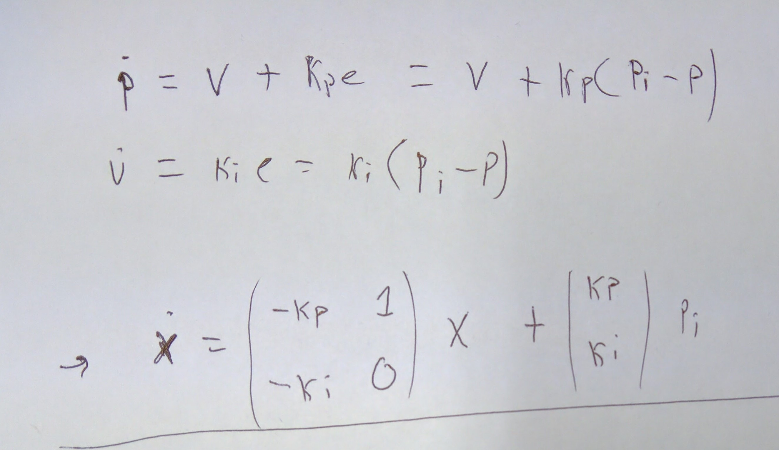
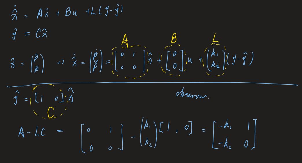
So the equations below we have two states p for position and v for velocity. For clairity I used a variable to e to mean the error between the position state and the encoder reading, the latter designated as p_i for “input position”. We can let a vector x be equal to [p, v], and hence write the two equations in matrix format.

Now you will have to trust me on this: the poles of this system is equal to the eigenvalues of the matrix on the left, the system matrix, commonly called A. (If you don’t trust me, check this).

Okay so what are the eigenvalues of the matrix? Back in the day you would have to go do some algebra, but with modern technology we can have computers do that for us: we use SymPy. Try it yourself at SymPy live. Enter this command: Matrix([[-x, 1], [-y, 0]]).eigenvals(). Pretend that x means Kp and that y means Ki. Voila, the solution is:

Going back to our specification: we want the real part of the pole to be some specific number, which is our bandwith (in radians/s) and we want the imaginary part to be zero on both poles. Solving for that yields:

IMG_20161218_211409_kpki

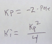
Which is exactly what is in the code:

motor->rotor.pll_kp = 2.0f * rotor_pll_bandwidth;
// Critically damped
motor->rotor.pll_ki = 0.25f * (motor->rotor.pll_kp * motor->rotor.pll_kp);
6 Likes

For anyone who wants to go a bit more deeply, go watch some of Brian Douglas’ videos.

2 Likes

You can improve the tracking error with torque feedforwad:
rotor->pll_vel += CURRENT_MEAS_PERIOD * TORQUE_CONSTANT * highpass(q_current) / MOTOR_INERTIA;

The highpass compensates constant load on the motor.

Yes, this is the plan as soon as we have automatic identification of load inertia.

i have a question. if the encoder has the resolution of 4096ppr/16384cpr. do we still need pll?

That’s just an observer constructed in such a way that the characteristic
equation of the observer is the characteristic equation matrix A-LC.

If the eigen values of A - LC are chosen properly, the error ( p_measured - p_estimated, v_measured - v_estimated) will be zero.

quick update